Labour income
The labour income module projects potential hourly wages for each simulated adult, paid-employment choices and gross labour income. Hours of work are generated for the adult members of a benefit unit, and gross labour income is calculated from hours worked and the corresponding wage rate.
Wage rates
Hourly wage rates are simulated using Heckman-corrected regressions stratified by gender and lagged employment status, distinguishing people who were and were not employed in the previous year. The explanatory variables include part-time employment, age, education, student status, parental education, relationship status, children, health and region. For people employed in the preceding year, lagged log hourly wages are also included.
Predicted wages are used for all individuals, rather than only for people who are not employed, because this approach performed better in model development. They provide the wage rate used to calculate employment income under each labour-supply alternative.
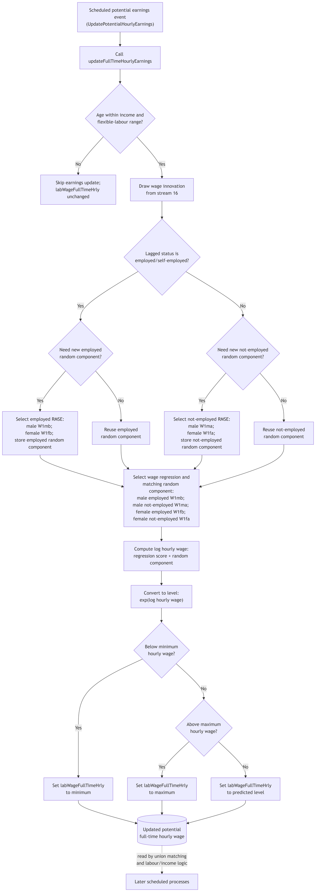
Potential-earnings diagram
This diagram records the implementation of the potential hourly-earnings update. It does not represent the complete labour-supply model.
View the potential-earnings diagram
Employment decisions
SimPaths provides two approaches to employment decisions. Both represent the influence of financial incentives, but they differ in whether expectations are treated as implicit or explicitly forward-looking.
Default within-period model
The default specification uses a non-forward-looking random utility model. Employment decisions are projected as though a benefit unit chooses from a discrete set of labour and income alternatives to maximise within-period utility. Utility is quadratic in benefit-unit disposable income and the hours worked by adult members.
The UK labour-supply model is estimated using UKMOD together with UKHLS data for 2019/20. Estimation uses an alternative-specific conditional logit model (asclogit in Stata).
Eligible decision units and alternatives
In the current implementation, labour-supply-flexible adults are aged 16 to 75 and are not students, retired or disabled. The lower bound is set by MIN_AGE_FLEXIBLE_LABOUR_SUPPLY. A flexible adult without a partner, or with a partner who is not flexible, is evaluated individually. Where both partners are flexible, their choices are evaluated jointly.
Each flexible adult chooses among seven mutually exclusive alternatives:
| Alternative | Representative weekly hours | Observed hours category |
|---|---|---|
| 0 | 0 | Non-employment |
| 1 | 10 | 6-15 hours |
| 2 | 20 | 16-25 hours |
| 3 | 30 | 26-35 hours |
| 4 | 38 | 36-40 hours |
| 5 | 45 | 41-49 hours |
| 6 | 55 | 50 hours or more |
For couples, the choice set contains every combination of the two partners' alternatives. The observed choice, simulated disposable income and calculated leisure identify the utility parameters.
Income and leisure under each alternative
Leisure is total weekly time minus the representative paid-work hours and hours spent providing care. Informal caregiving therefore enters the utility function as a time cost.
For each hours alternative, the predicted hourly wage is used to calculate employment income and UKMOD calculates disposable income. The counterfactual calculations follow four conventions:
- Taxes and benefits that UKMOD can simulate, including Universal Credit and tax credits, are recalculated for every alternative.
- Benefits that UKMOD cannot simulate and that depend on employment income are set to zero in counterfactual alternatives. Otherwise, they would appear only in the observed alternative and distort utility estimation.
- Benefits that UKMOD cannot simulate, do not depend on employment income and are compatible with work retain their observed amount in every alternative.
- If a benefit received in the observed state is incompatible with work and makes some alternatives infeasible, the person is excluded from the estimation sample where required.
Estimation groups and utility specification
The estimation sample distinguishes:
- single women;
- single men;
- couples in which both partners are flexible;
- women with a non-flexible partner;
- men with a non-flexible partner;
- adult daughters; and
- adult sons.
Limited sample sizes require the sexes to be pooled for adults with one flexible partner and for adult children.
Utility is quadratic in disposable income and leisure. The single-woman and single-man specifications include a full-time-work indicator and years spent in employment. The couple specification includes full-time-work indicators and previous labour-market experience for both partners. For adults with a non-flexible partner, men and women are estimated jointly and the full-time-work indicator is interacted with sex. Adult children are also pooled with a sex-by-full-time interaction, but previous labour-market experience is omitted because it was not statistically significant.
Forward-looking specification
The model can instead project labour supply and discretionary consumption using explicit forward-looking expectations. The unit of analysis remains the benefit unit, and incentives are translated into behaviour through an intertemporal utility function. By default, this is a nested constant-elasticity-of-substitution utility function.
Each adult has three labour-supply alternatives: full-time work, part-time work and non-employment. Labour supply and discretionary consumption are projected as though they maximise utility subject to a hard constraint on net wealth and the agent's expectations. Expectations are substantively rational: uncertainty is represented by the random processes driving the dynamically projected characteristics.
Because the lifetime problem has no analytical solution, it is solved numerically in two stages. First, the model solves the lifetime decision problem for possible combinations of relevant agent characteristics and stores the solutions in a look-up table. During the simulation, the appropriate stored solution is used to project labour supply and discretionary consumption.
Alignment
Under the default labour-supply specification, the estimated utility of single men, single women and couples is adjusted so that aggregate employment rates follow observed rates during the validation period. The final adjustment is retained in later periods for which no observations are available. This procedure partly accounts for unemployment and labour-demand constraints that are absent from the unconstrained random utility model.
Technical implementation
Annual ordering is coordinated by SimPathsModel. Person-level wages and employment states are held in Person, while joint decisions and income calculations are coordinated at BenefitUnit level. Parameter files are summarised under Model Parameterisation.